
Risk is one of the greatest enemies against growing and protecting your assets. There are two forms of risk: Unsystematic and systematic risk, write Pranav Singh and Brad Reinard, chief publishers at Monthly Cash Thru Options, an options advisory newsletter and educational service.
(Sponsored content) Systematic risk, also known as market risk, is caused by inflation, geopolitical events, and broad macro events. This type of risk can move entire sections of the market, such as the large-caps, specific subsets of an asset class, or the entire market itself. Systematic is difficult to evade due to its wide spread effects and unpredictability.
Alternatively, unsystematic risk is caused by events or actions from specific companies, industries, or investment strategies. Unsystematic risk can be addressed through diversification. This article outlines a methodology that can be used to develop a diversification strategy to mitigate unsystematic risk.
To effectively diversify an investment portfolio to mitigate unsystematic risk, one can combine complimentary assets or strategies that will counteract one another. This approach of reducing risk is based on Modern Portfolio Theory that states that combining two or more complimentary assets can improve the returns for a given level of risk. The classic example of balancing complimentary assets is to blend stocks with bonds.
When determining the compatibility of two assets, one tool within the framework of Modern Portfolio Theory to analyze the effectiveness of diversification is the efficient frontier. The efficient frontier compares returns of each asset over a respective holding period versus a risk metric, such as standard deviation, across different allocation levels. For this example, we look at a strategy that balances the S&P 500 Index ETF (SPY) for the equity holding and the iShares Barclays 20+ Year Treasury Bond ETF (TLT) for the bond holding.
Before we plot the efficient frontier for our example portfolio of the SPY and TLT, let’s first review what standard deviation is. Standard deviation (SD), in this case for an investment portfolio, represents the average dispersion of returns and is a typical measure of risk. Let’s go through the process of calculating the SD for the SPY.
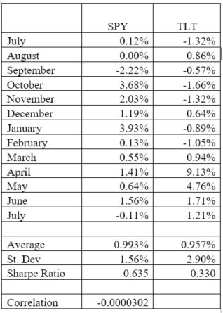
The table below shows a sample of monthly returns for the SPY and TLT from July 2016 to July 2017. We will use these values as sample values for the example portfolio moving forward.
To calculate the SD for the SPY we use the following formula, which is specific to calculating the SD for a single asset:
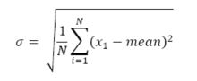
Where N is the number of monthly return values.
First, we calculate the mean of the SPY returns by summing the returns and dividing by 13, which is equal to 0.993%. Next, each value is subtracted from the mean and squared. Finally, we calculate the average of this new set of values and take the square root of this final mean resulting in a SD of 1.56%. A standard deviation of 1.56% can be interpreted as the average dispersion of the monthly return. In statistical terms, assuming a normal distribution, we can expect the returns to fall between -.567% (0.993 – 1.56) and 2.55% (0.993 + 1.56) sixty-six percent of the time.
Following the same steps shown above, the SD for the TLT is 2.9%. These values can be easily calculated through the Excel function STDEV.P. An observation for these individual assets is that both the SPY and TLT have similar average monthly returns near 0.97%. However, the dispersion of the returns for the TLT is larger, coming in at 2.90% versus 1.56% for the SPY. Thus, the returns are similar, but the risk during this period was higher for the TLT.
We now combine the SPY and TLT into a single portfolio to see if the SD of the combined portfolio is less than either of the above two values.
To calculate the SD of a two-asset portfolio we use the following formula:

Covariance is a measure of how changes of one variable are associated with the changes of a second variable. In other words, covariance quantifies how closely two assets move in tandem. It is calculated as follows:
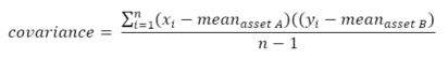
In Excel the function used to calculate covariance is COVARIANCE.P. The covariance value is what makes diversification effective. Any two suitable assets will at times move against each other. This is captured in the covariance and as the value becomes more negative the SD of the portfolio will decrease.
After calculating the SD, we use this value to calculate a comparable measure of risk called the Sharpe ratio. The Sharpe ratio is calculated by dividing return by risk and represents normalized, “risk adjusted returns” of a portfolio. By using a normalized metric like the Sharpe ratio, we can more easily and accurately compare different assets and portfolios. When analyzing varying weightings of the assets within a portfolio of two or more assets, the highest value of the Sharpe ratio represents the most optimally weighted portfolio with the best risk adjusted returns.
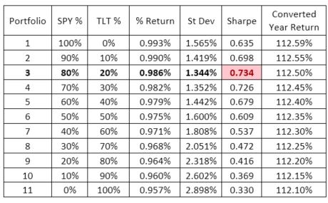
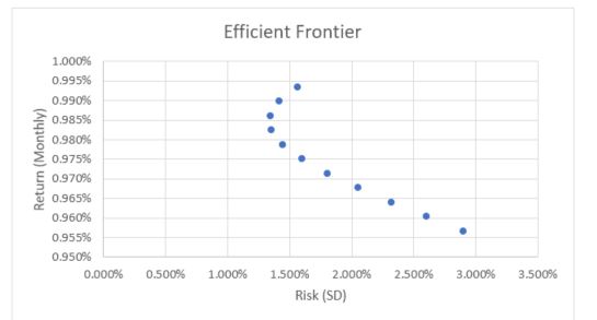
In the table shown below we analyze varying weightings of the SPY and TLT ETFs within our hypothetical portfolio. Portfolio #1 comprises 100% of the SPY where it increased an average of .993% per month with a SD of 1.565%. On the other extreme, portfolio #11 comprises 100% of the TLT where it increased at a similar .957% per month, but with a SD of 2.898%. We can see that portfolio #3, with an 80:20 distribution of the SPY and TLT, respectively, represents an optimally weighted portfolio with a 0.986% return, 1.34% standard deviation, and the highest Sharpe ratio at 0.734.
Let’s compare the risk and return values of the portfolio to the individual assets. The Sharpe ratio for each asset is .635 and .330 for the SPY and TLT, respectively. The Sharpe ratio for the portfolio is larger, telling us that risk adjusted returns are better with the combined portfolio versus the individual assets. Moreover, the 80:20 weighting reduced the SD, or overall risk, to 1.34% vs. 1.57% for SPY and 2.90% for TLT, a 36.3% reduction in risk. The return remained the same at .986%. As shown numerically the multi-asset portfolio effectively reduces risk by a large margin while quantifying the maximum possible return for a given level of risk. In the long run an investor can expect to outperform any of the other portfolios since risk is reduced while not compromising the returns.
Below is a graphical representation of the SD and monthly return values for the SPY and TLT portfolio that creates the efficient frontier. We can see that the left most data points represent the optimal portfolios with the best risk-adjusted returns.
The most important takeaway from our analysis is that diversification works, thanks to covariance. The stronger the effect of covariance on the portfolio’s SD, the more an investor will be able to reduce risk for an optimized level of return. This effect is amplified with better pairings of assets that have more negative covariance, and by adding more assets. Similar to how this technique was applied to the SPY and TLT, one can create a myriad of multi-asset combinations to achieve high Sharpe ratio portfolios. For instance, an option credit spread strategy paired with a long-only equity strategy may provide a high Sharpe ratio. Another example is blending U.S. based assets with international funds to maximize returns while retaining the stability of U.S. economy. The possibilities are endless, and the efficient frontier is one tool that makes choosing complimentary assets easier and more effective.
About the authors: Pranav Singh and Brad Reinard are Chief Publishers at Monthly Cash Thru Options, an options advisory newsletter and educational service provider. For more information about the MCTO services and investment track record please visit www.monthlycashthruoptions.com. You may also contact Pranav directly at pranav@monthlycashthruoptions.com, or Brad at brad@monthlycashthruoptions.com