
Last week Paul Cretien introduced the log log Parabola (LLP) Options Pricing Model. Here we explain how it works.
The log log parabola (LLP) pricing model is a regression analysis that produces a price curve of predicted option prices given the market prices of options in a chain of strike prices. The two Ls in the name stand for the two series of natural logarithms that create the price curve.
Although it looks complicated, the LLP model is not a theoretical program. However, the options prices from which it computes a price curve are generally based on theoretical models that determine option prices given underlying economic and market values. It happens to be true that the market prices form log-log parabolic curves.
Once a price curve has been computed for an options price chain, the call or put option at each strike price is shown to be over-priced or under-priced relative to the predictive price curve. Trades can be based on variances of option prices around the predictive curve, with the assumption that a relatively large variance – plus or minus – will be the cause of price movement back toward the price curve, i.e. reversion to the mean.
The words “stock” and “underlying asset” are used here to mean any asset for which options are being calculated. These could include stocks, futures, U.S. Treasury securities, exchange traded funds (ETFs), currencies, etc.
The asset’s market price is entered in column A. The program currently copies the price into all the cells in column A. However, it would be possible to enter data from several times or days, or to enter data over several time periods to have a moving average price curve. Enter the number of strike prices used in cell B3.
For call options, use the highest strike prices leading down to the strike equal to or just above the asset’s market price. For puts, use lower strike prices leading up to the stock’s price. At least three strike prices are needed for either a put or call since three points determine a curve. If there are many strike prices available you may want to skip some; for example use every other strike price. Also, some weeding out of options that are obviously miss-priced by the market is sometimes necessary. It is not necessary to include an option that would distort the price curve.
When all of the option prices have been entered in column C for the strike prices you have selected, column D will show the calculated predicted price curve. We show how it is calculated using Apple (AAPL) options (see table).
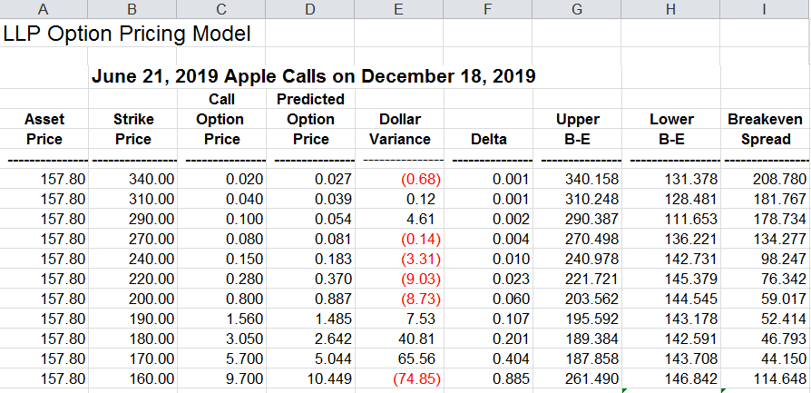
Column E will compute the dollar amount of the variance between each option’s price and the predicted price. The difference between columns C and D is multiplied by the dollar value of one option point. You will enter the value per option point in cell G3. For stocks (equities) $100 per point is used in this model. For other assets the dollar value per point varies. For example with calls and puts on Swiss francs the value of each option point is $125,000. For those currency options the dollar variances are very small even with the large price per point.
Delta values in column F show the slope of the price curve at each strike price. The slope of the change in the option’s price for each unit change in the asset’s price. The delta values are used in columns G and H to calculate the upper and lower breakeven (profit or loss) from a “delta neutral” trade – selling the number of calls equal to the inverse of the delta ratio, and multiplying this number times the price per call option, and at the same time taking a long position in the underlying stock (or asset).
The delta trade formulas should be used only for calls. The formulas are not designed for puts.
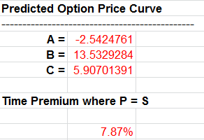
Directly below the computed price curve’s A, B, and C coefficients at the bottom of the page is the time premium. This premium percentage may be used as a means of comparing volatilities between companies, currencies or other classes of assets.
The best use for the LLP model is in finding price variances (column E) large enough to profit from a return of over-priced or under-priced options to the predicted price curve, above the cost of the trade.
Another use for the model is to show the effect of a change in the market price of the underlying asset while using the same price curve. Going to the A. B, and C coefficients in Column AA, the formulas could be copied to one side to be available to copy back sometime later. Then the A, B, C values in Column AA could be “frozen” by using the “paste special” command with “values.” With the price curve frozen, a new stock price would result in new predicted option prices but on the original price curve – thus showing the effect of a change in the underlying asset price. This is valuable because the computed price curve should be relatively stable for several days, while the stock price may have large changes.
For assistance or questions regarding the LLP Options Pricing Model, contact Paul at Cretien619@aol.com
I would appreciate your ideas and experience using the model.